
TLDR; A write up of an assignment from Coursera’s Data Analysis course aiming to identify patterns of activity from accelerometer data using SVD and Randrom Forests in R.
I’ve been following Coursera’s “Data Analysis” course, taught by Jeff Leek (straight outta Hopkins!). It’s been interesting, having spent 7 years doing particle physics, most of the techniques are not new, but the jargon is. It has also highlighted some important differences in the methodology of Particle Physics and Bio-statistics, driven by our reliance on synthetic data (or conversely, driven by their lack of reliable Monte Carlo). Since the second assignment is over and done with, I thought I’d post a little write-up here.
The aim was to study the predictive power of data collected by the accelerometer and gyroscope of Samsung Galaxy S II smartphones, carried by a group of individuals performing various activities (walking, walking upstairs, walking downstairs, sitting, standing, and laying down). The dataset consists of 7352 samples (pre-processed by applying noise filters and by sampling the values in fixed time windows) of 562 features collected from 21 individuals. Of these 21 individuals, I randomly set aside three as a testing sample, and another four as a validation sample.
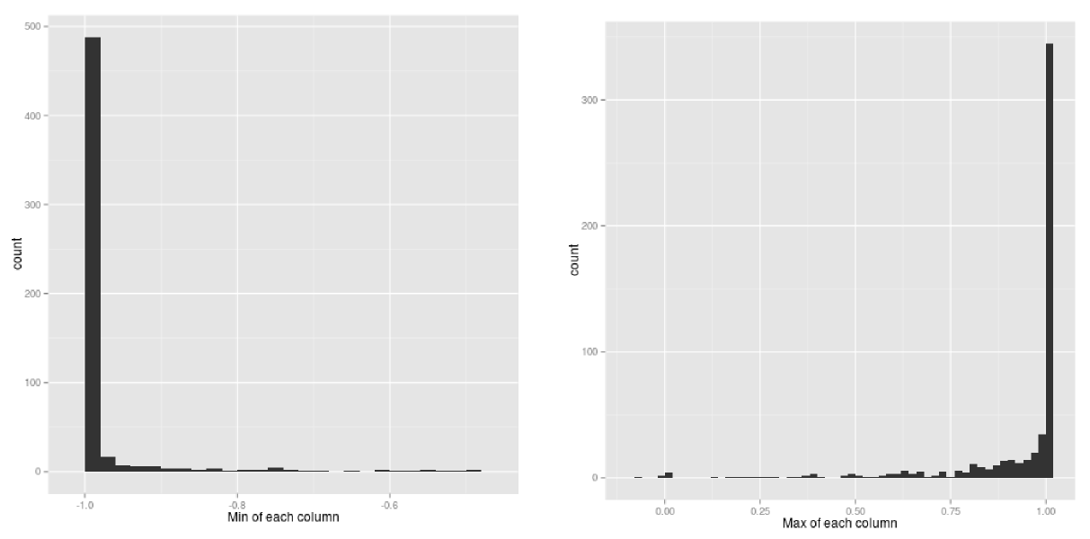
This data is relatively well behaved, each activity is represented about equally in the dataset, and the range of values spans [1,-1] in all cases. Though some variables have asymmetric distributions, none appear to require a transformation between logarithmic and linear scales. There are a number of variables with bi-modal distributions, mirrored around 0. Since this is often an indication that the sign of the distribution carries meaning, I appended a copy of each variable’s absolute values to the dataset to later ferret out any sub-leading effects.
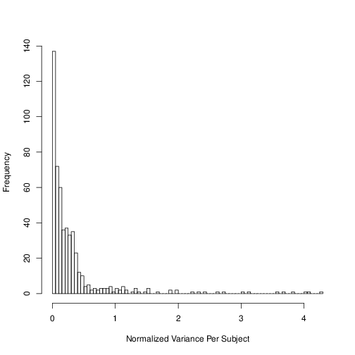
In any study involving classification, it’s important to identify whether potentially discriminating variables are healthy out of sample. In plotting the training set readings, it became apparent that some variables do not behave the same for all subjects (the means or variances of the variables for a given subject can be very different). From the available information, it is not clear whether this could be caused by some difference in the physical health of the subjects, or whether the data is itself somehow corrupt. Regardless, it’s best to try to identify these kinds of effects, and avoid using those variables if possible. A good method to systematically quantify this effect is the absolute normalized variance per subject (V_{ij} = abs(var(x_{ij} )) / mean(x_{ij})), where V_{ij} is the variance of the ith variable for the j th subject, and x_{ij} is the set of values for the ith variable. While the bulk of variables behave the same across subjects, there is a long tail, and generally variables with V_{ij} > 1 are likely to introduce variance in the predictions, even if they improve the in-sample fits.
As I mentioned earlier, there are 562 features per sample (1124 after storing their absolute values), most of which likely do not carry much discriminating power. Obviously, I had no intention on investigating each of those variables individually. But rather than go in, guns blazing, with some dimensionality reduction technique, I decided to use Singular Value Decomposition (SVD) to identify the original variables which contain the most variance.
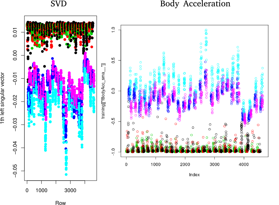
One of the nice things about SVD is that, while it can generally construct a lower-rank description of the data, it’s also possible to identify the source rows (or rather, variables) which span the data space. If you’re lucky, this means you get to maintain most of your descriptive power, and still operate in a less abstract basis. In this case, it’s easy to split apart active and passive activities and a cut on just one variable identified by SVD (the acceleration magnitude measured by the device) nets you about 99% sample purity. The rest requires some more finesse.
By further sub-setting the data and again performing SVD, a dozen or so additional useful variables emerge. Unfortunately, there is no silver-bullet for separating activities like walking up stairs from walking down stairs. A combination of several variables gives some hope. However, there’s a lot of mutual information in the variables identified by SVD. The use of mutual variables is something that we try to minimize in physics analyses for a variety of reasons, not least of which is that they introduce extra work for little gain (and we physicists are notoriously lazy).
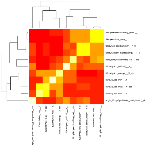
A correlation matrix of the variables quickly reveals which ones have strong (linear) dependencies, and thus which ones we can drop with little loss in discriminating power. We’re left with a dozen of so variables which our foray into SVD tells us should be highly descriptive of our subject’s activity. This now looks like a text-book classic problem for an old standby, random forests. These guys are great at classification, can approximate high-order functions, and by construction don’t (or at least avoid) over-fitting the data. Their output is something of a black-box, but by this point, the data and the variables seem under good enough control that I don’t consider this a problem. I trained two types of trees, one in which a greedy-selection algorithm adds all the “good” variables which improve the performance of the classifier, and a second one in which I manually selected a subset of the variables. While the mechanism which trains Random Forests can also report an out-of-bag error rate, which is usually a pretty good estimate of the true error, nothing beats k-fold cross-validation (where in this case k = 10). Remember how I said we usually try to minimize the number of input variables in physics analyses? Well, here’s an example of one of the well-motivated reasons. The greedy random forest has an out-of-bag error of 1.3%, almost half the k-fold error of 2.3%. Conversely, the random forest with the hand-selected variables claims an out-of-bag error of 2.1%, compared to a 2.3% k-fold error.
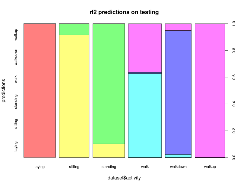
Of course, the error is not uniform across the activities, as always, the devil is in the details. Opening the box and applying the random forests to the test set, the final error is 4%. A factor of two off from the expectation might seem bad, but given the statistics, this is actually a somewhat reasonable result. It’s, certainly within the 95% confidence intervals of the expected error, and I’m going to use that as an excuse not to dig too much deeper into this (I do have a day-job after all).
So there you have it. There’s probably more performance that could be eeked out by using some clustering techniques, either to identify other important variables, or to generate entirely new features. But, I’d say this isn’t too bad for a few hours work 😉